This is a course project of CSE6730 @ Georgia Tech. The time span for this project is 30 days.

Visit the github repo of the project
Visit the playback demo of the project

Simulation-DES project for Tech Square Intersection Traffic

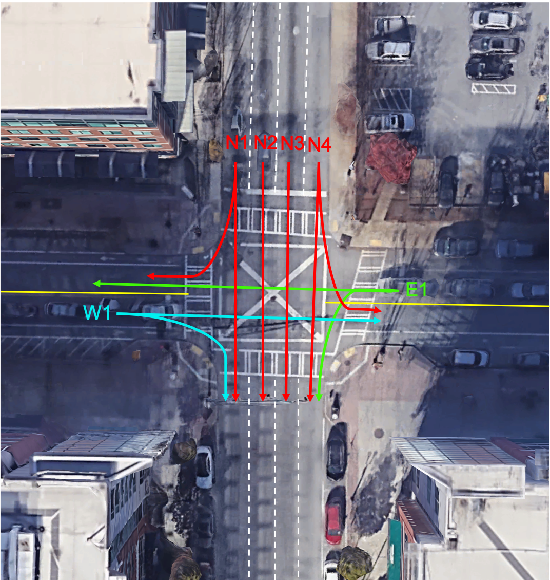
@Georgia Tech, Tech Square Intersection : View on Google Map: Spring St NW & 5th St NW, Atlanta, GA

Introduction

The intersection between Spring Street and 5th Street (Tech Square) has been one of the busiest area on Georgia Tech campus. Students are rushing to classrooms from main campus and vehicles are taking Spring Street to Interstate Highways. The traffics lights control is vital in this heavy traffics area for both protecting the safety of pedestrian and improving the efficiency of traffic flow.
In 2018, a new traffic pattern is introduced by including a “pedestrian scramble crossing” as known as Barnes Dance, where the major improvement is that introducing a “all-way-right cycle” for vehicles and pedestrians can cross this intersection in any direction.
This project will simulate this new traffic pattern with a discrete events simulation (DES) to study and further improve current system of traffic control.

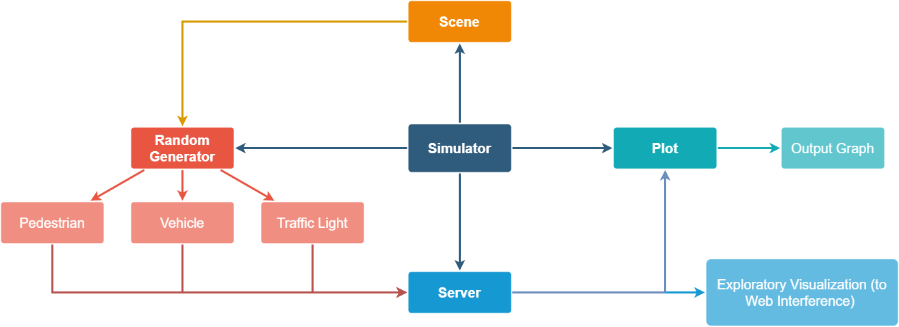
Software Architecture

Installation

1. Install the complete software package:

   git clone git@github.com:MUYANGGUO/Simulation-DES.git
   

2. Install the visualization dependencies

   cd ~/.../Simulation-DES/Visualization
   npm install
   

   note:
   The Visualization is a react.js web page application, it needs node.js installed. The dependency packages need to be installed with npm install. The Visualization also depends on the Simulation results. The simulation python software package will generate a test.json file which will overwrite the current test.json in Visualization folder.

Run Simulation

cd ~/your location path/Simulation-DES
python3 simulator.py N P T

N: Number of vehicle events within time duration, P: number of people events within time duration (unit is “crowd”) ,T: Time duration (hr).
Note that you should come up with these two number starting with the expectation of the events/per unit time rate, as the model will apply a poisson random process to simulate the observed occurrence of events within the time duration. The sampled observed events rate will be close to the expectation rate.

help line for understanding the software inputs:

python3 simulator.py -h

And the helper function will show:

usage: simulator.py [-h] total_events total_people simulation_time

positional arguments:
  total_events     :indicate the total events would like to simulate,
                   requested here
  total_people     :indicate the total people would like to simulate,
                   requested here
  simulation_time  :indicate simulation duration time, unit is hour, requested
                   here

optional arguments:
  -h, --help       show this help message and exit

Run Example:

python3 simulator.py 150 4 0.1 >output_test1.txt

The command window will print out the configurations info and reminders, once the program complete, an output folder will be generated for saving plots.
If with >output.txt added, the system output will be saved in this text file. If without this, the system outputs will pop out in the command window.

Run Visualization

After getting the test.json (will be stored in the visualization folder) from running simulator.py in the upper level directory, cd to Visualization directory, and run the following command:

npm start

The localhost will be started, and a web browser with the visualization page will be shown up.

Animation speed setting:

The animation cycle time, looplenth should be based on your simulation time duration (unit: second). If you run the simulation over 1 hour, you should set this number at least 3600.

The animation speed is the scaled up playback speedup. You can set any number to increase the time lapse speed for playback.

In app.js line 75.

  _animate() {
    const {
      loopLength = 360, // unit corresponds to the timestamp in source data
      animationSpeed = 2 // unit time per second
    } = this.props;
    const timestamp = Date.now() / 1000;
    const loopTime = loopLength / animationSpeed;

    this.setState({
      time: ((timestamp % loopTime) / loopTime) * loopLength
    });
    this._animationFrame = window.requestAnimationFrame(this._animate.bind(this));
  }

Output Figures

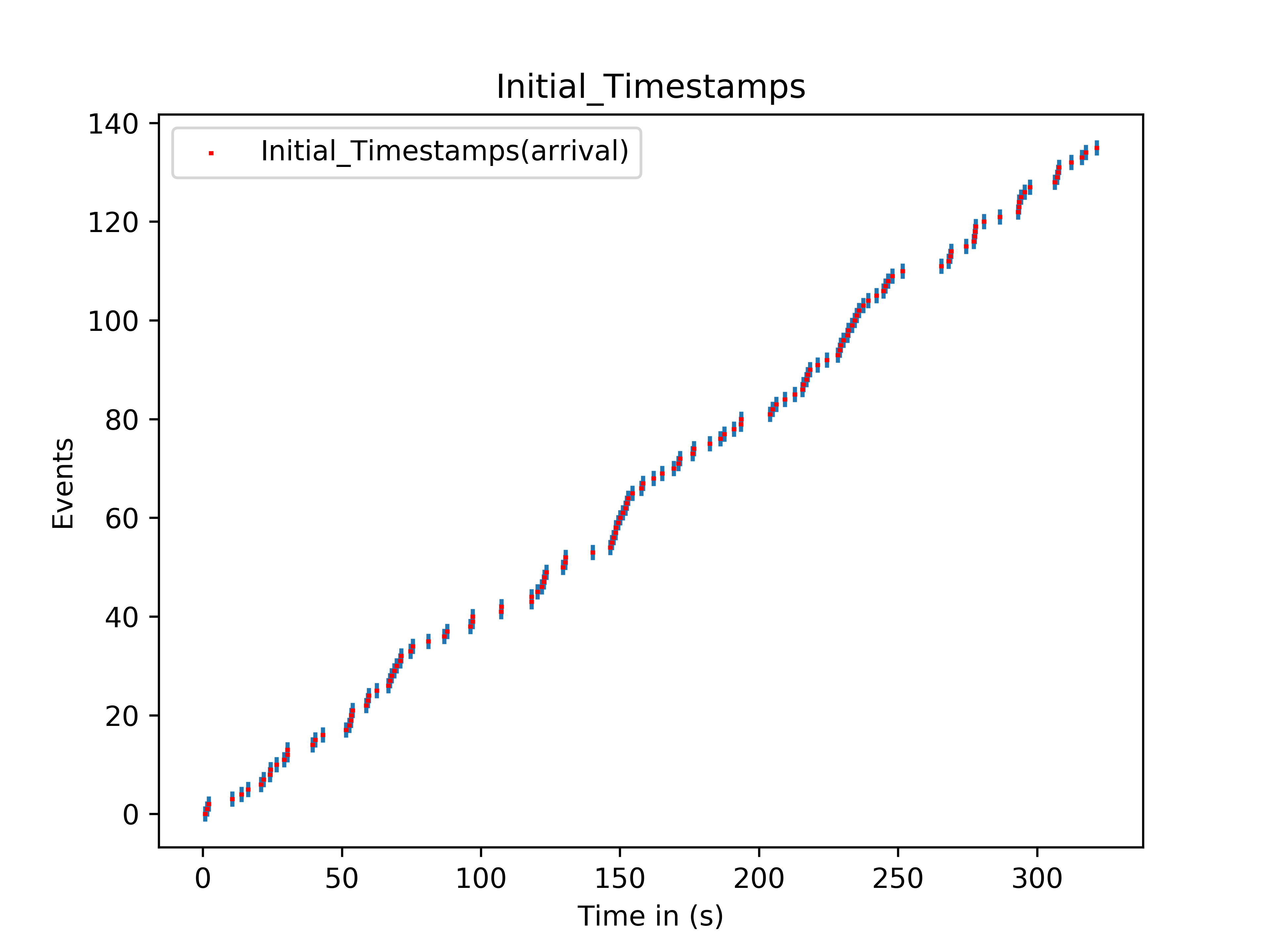
Output figures will be saved under generated outputs folder at the end of the simulation process.

1. Initial Poisson Distribution of Events Generating
The poisson distribution random genrator can be referred to my blog here which verifies our poisson generators outputs.
My Poisson Distribution Generator and verification histograms

2. Initial Arrival Timestamps for actors

3. Initial Each Lane Assigned for actors

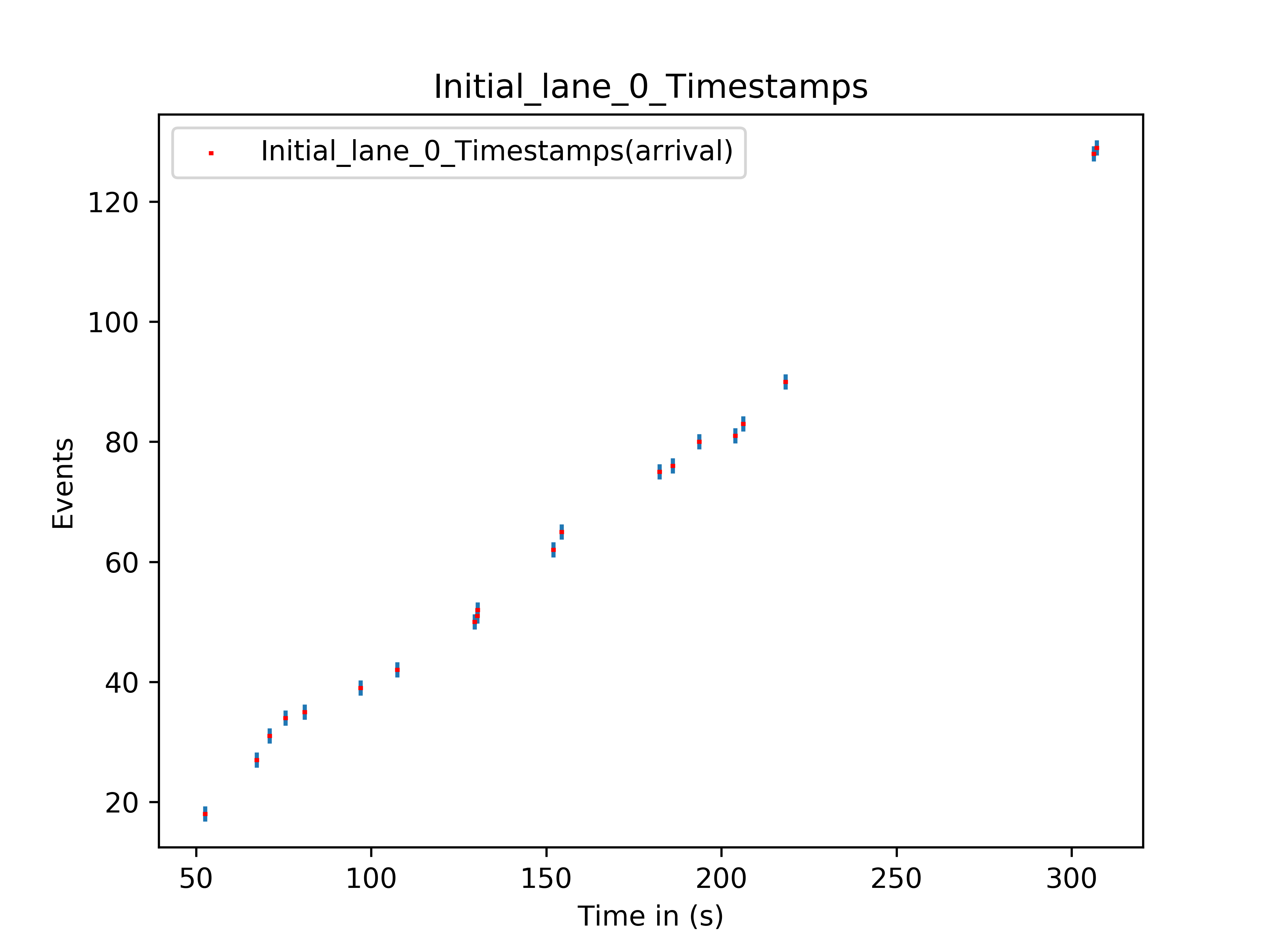
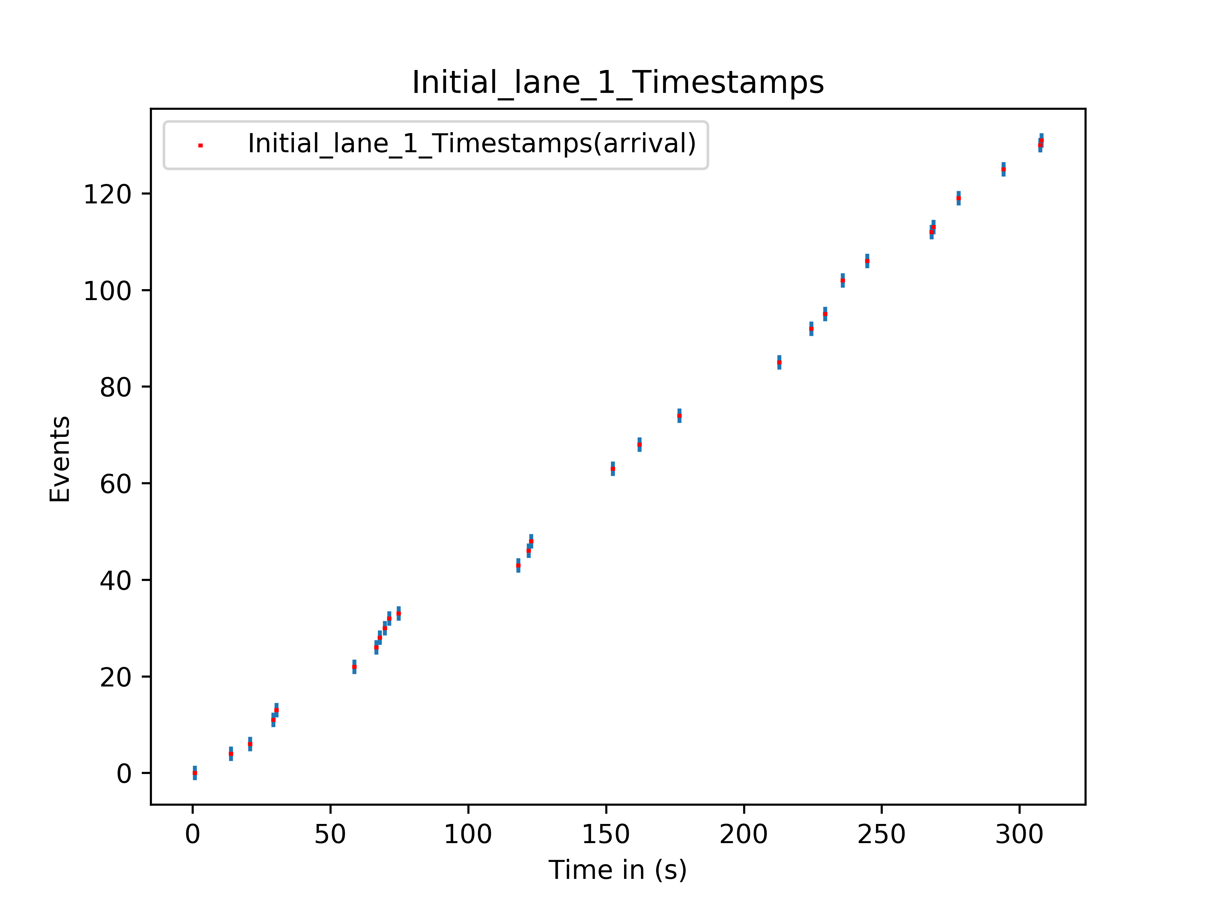
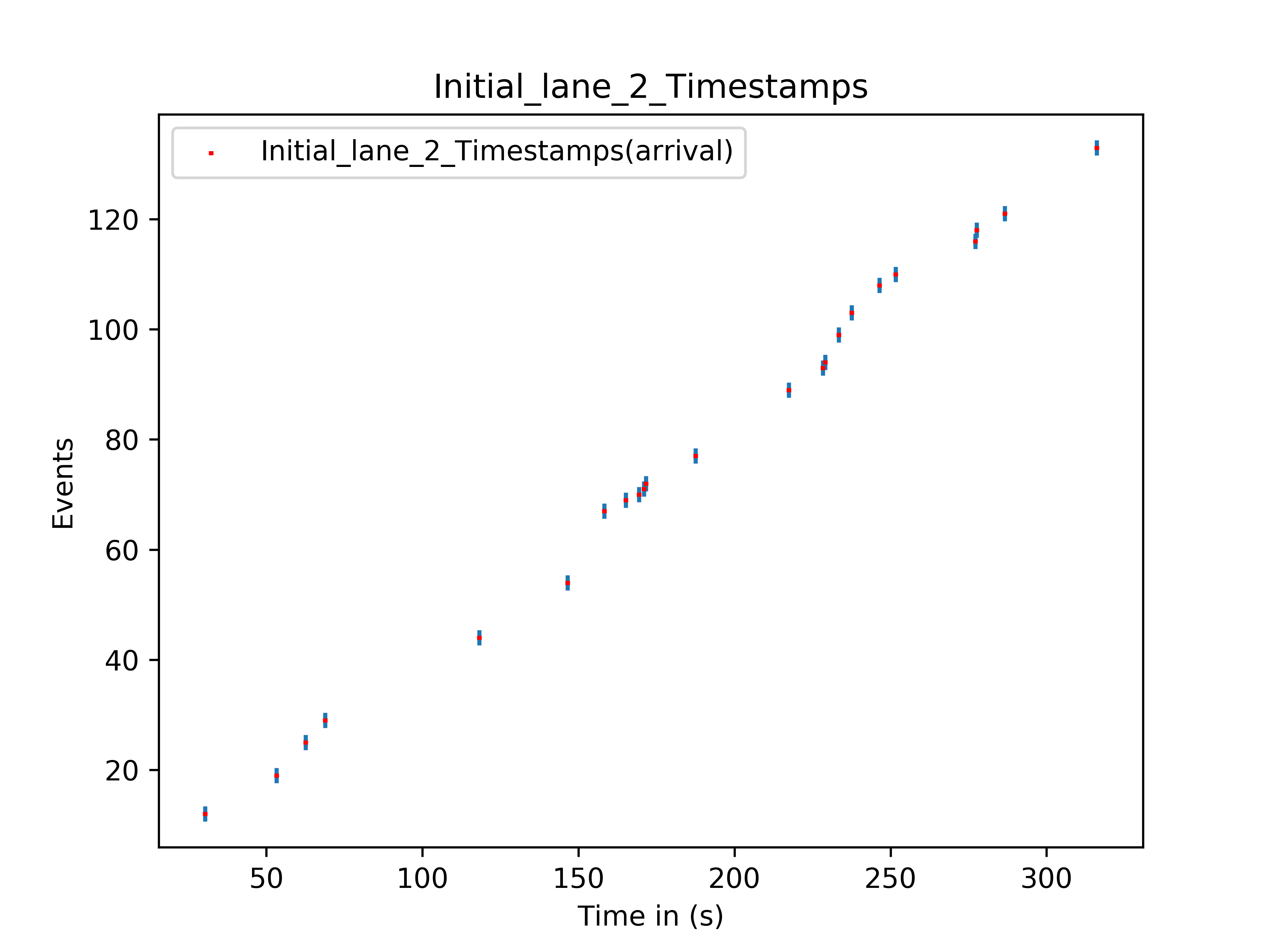
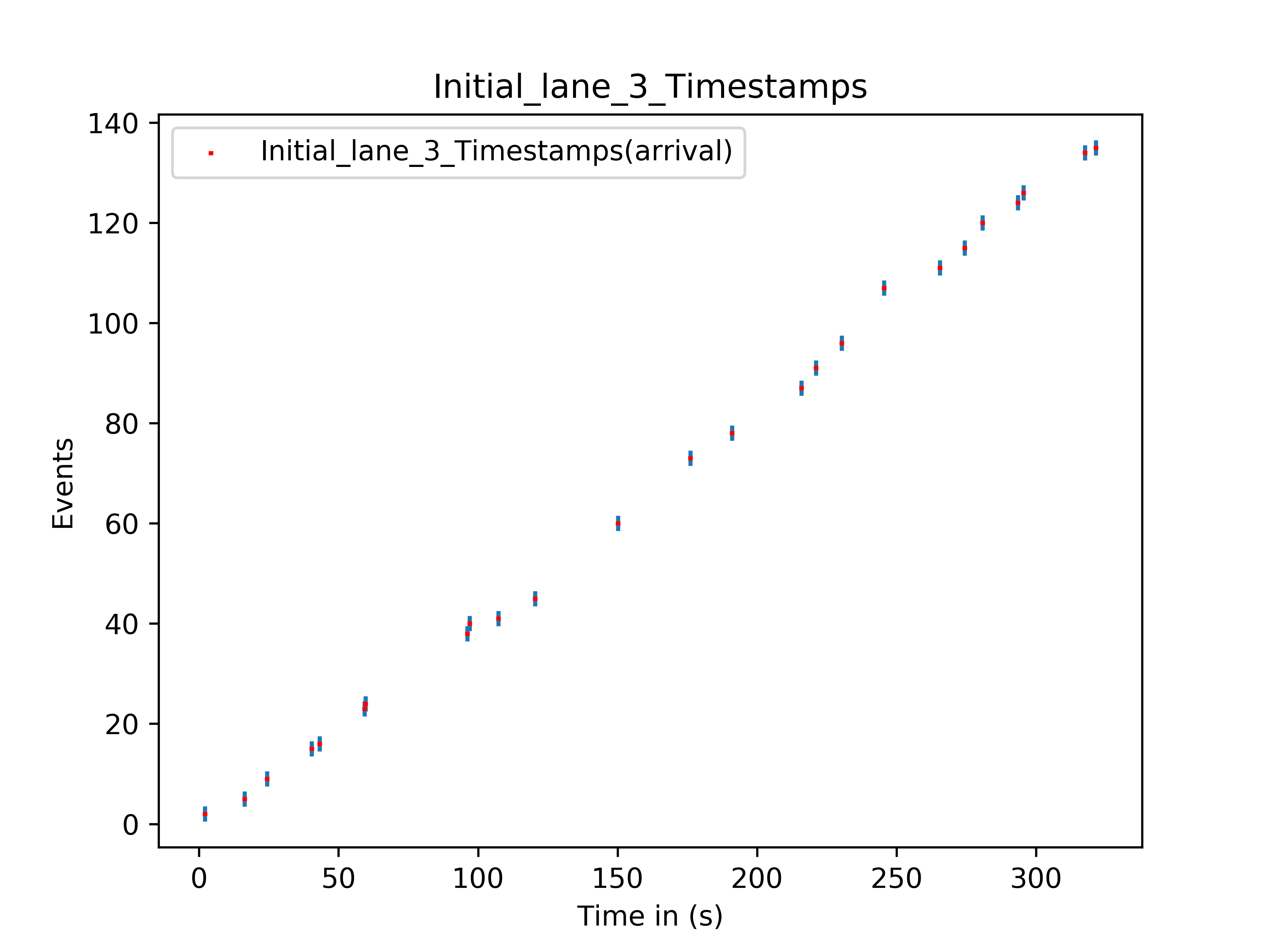
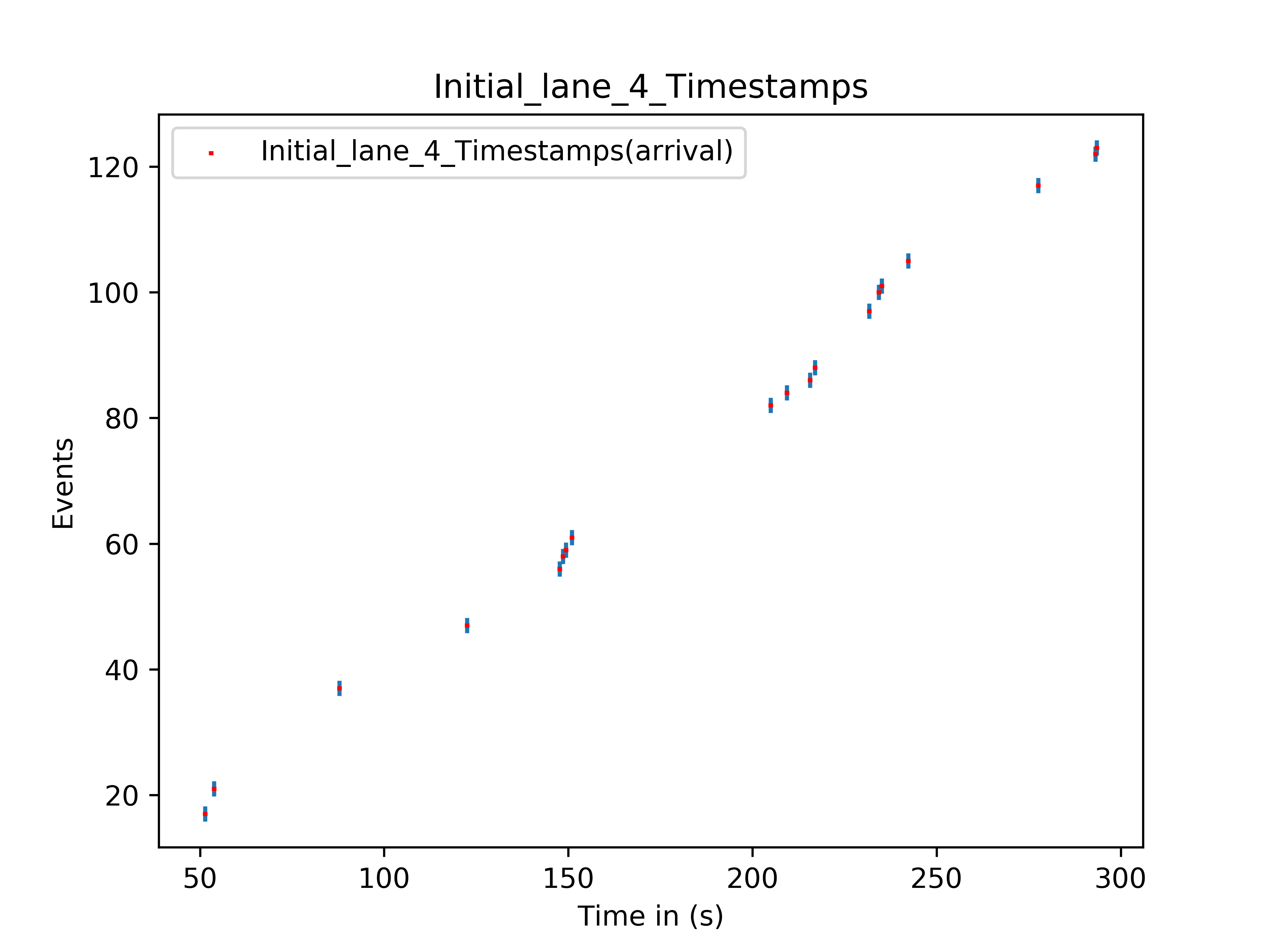
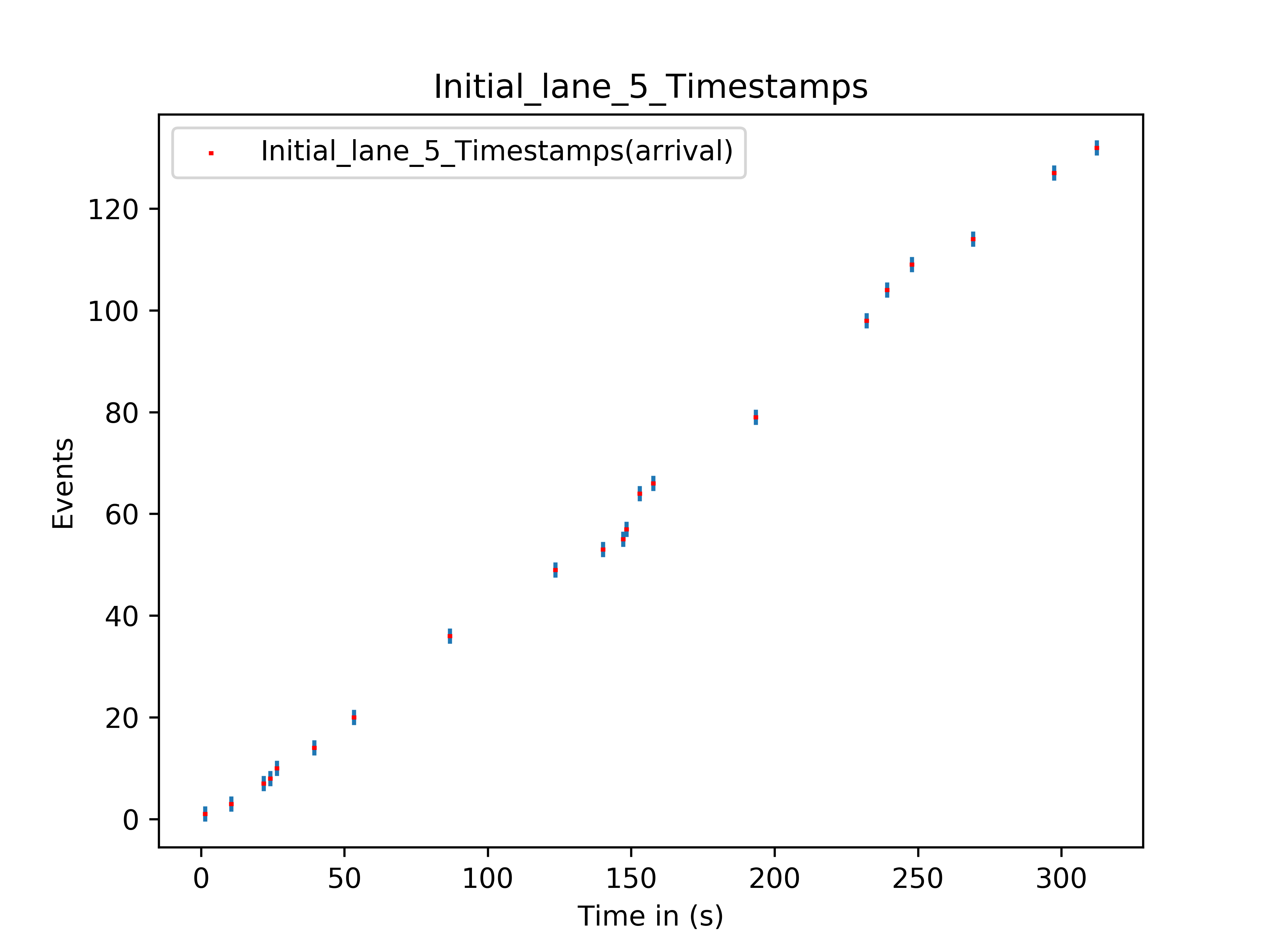
4. Final Each Lane Arrival Timestamps

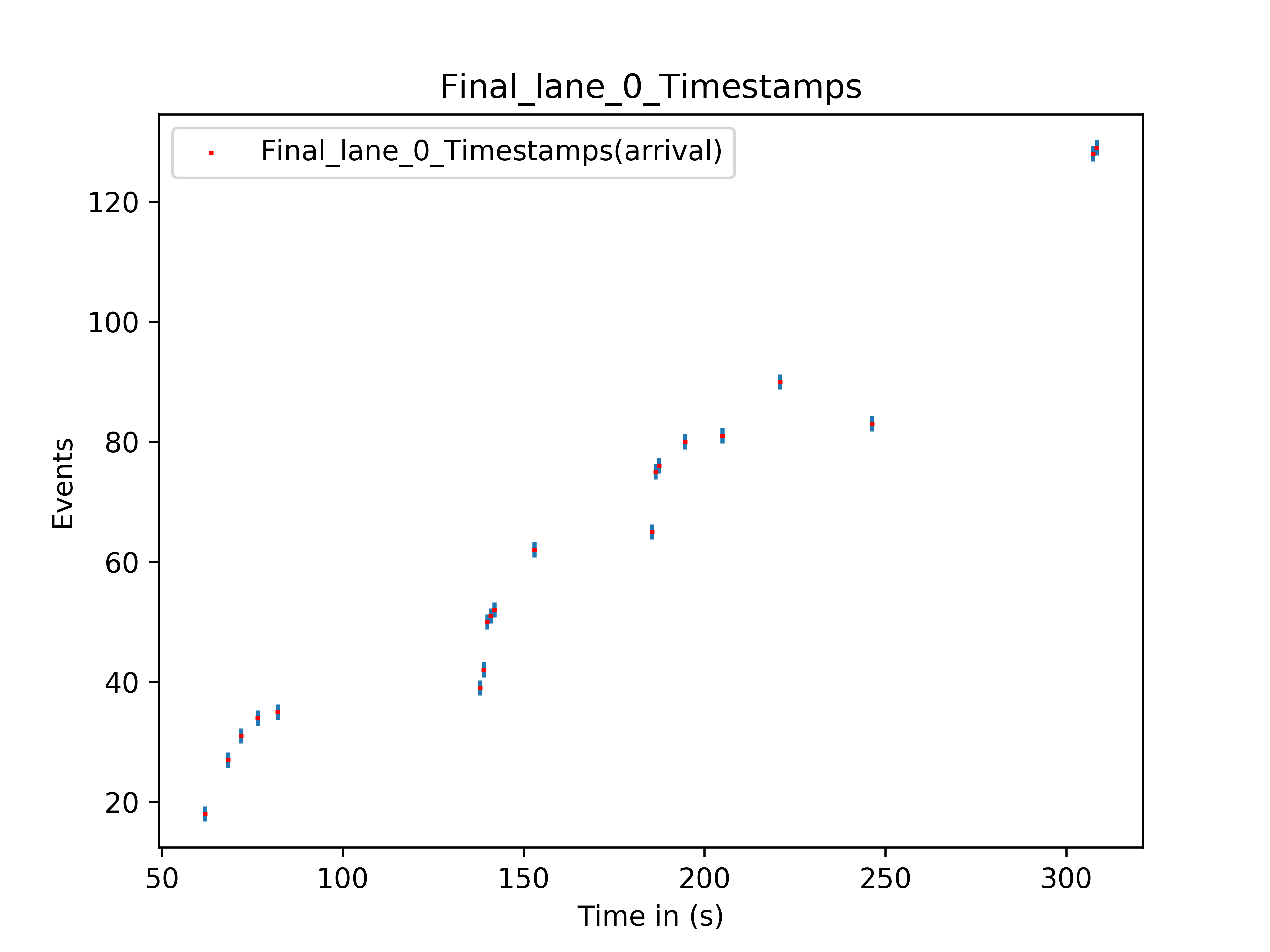
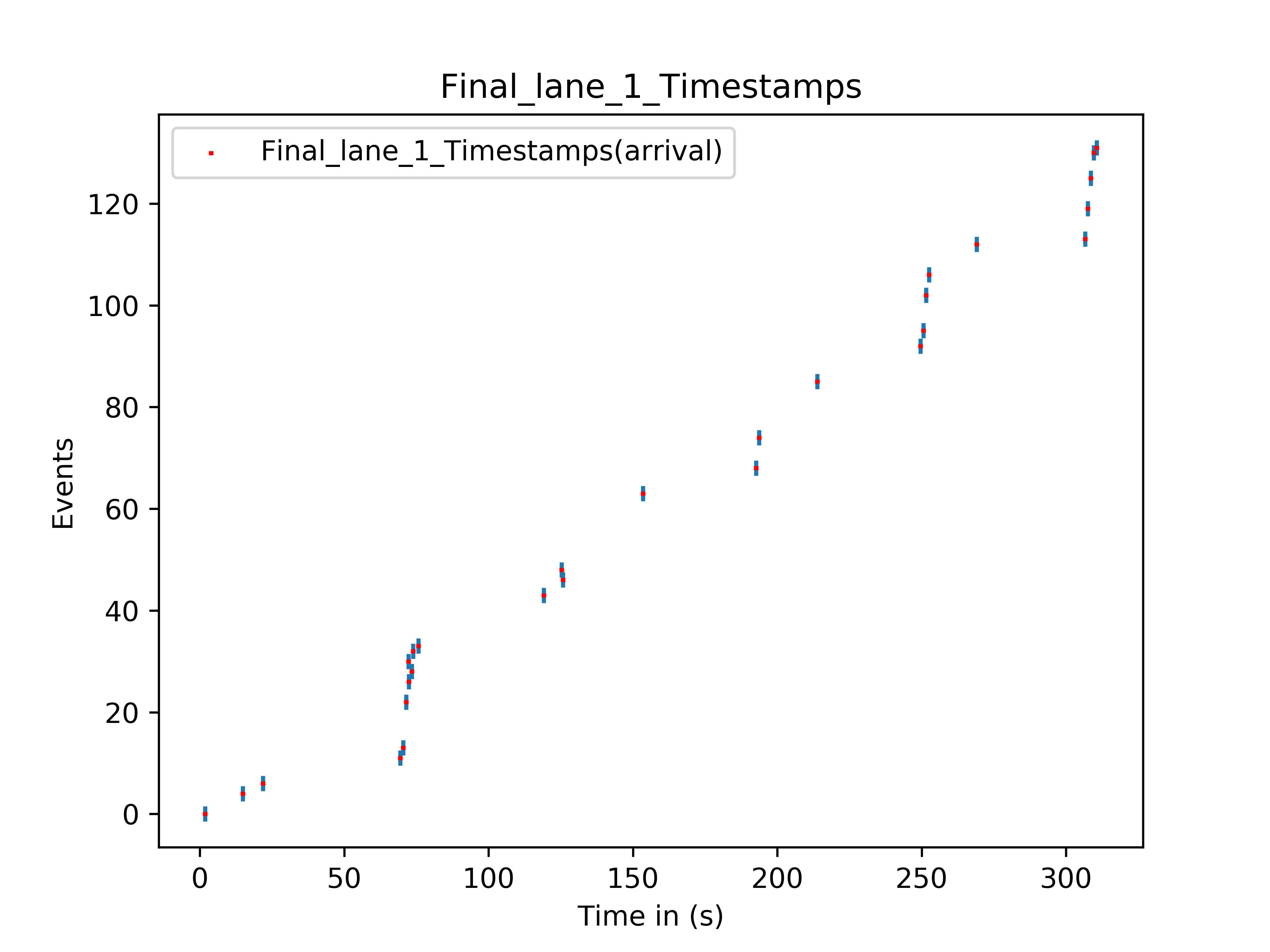
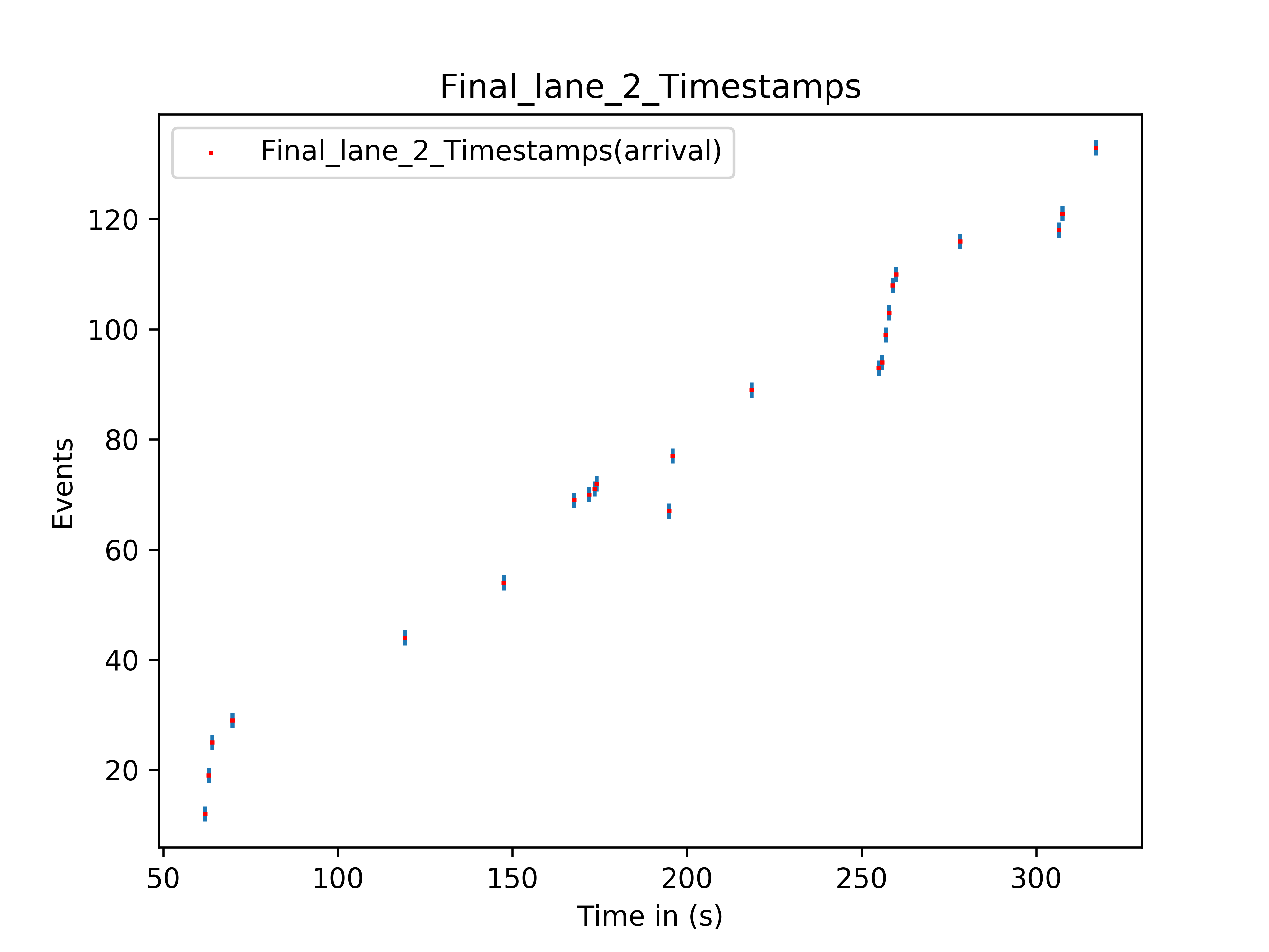
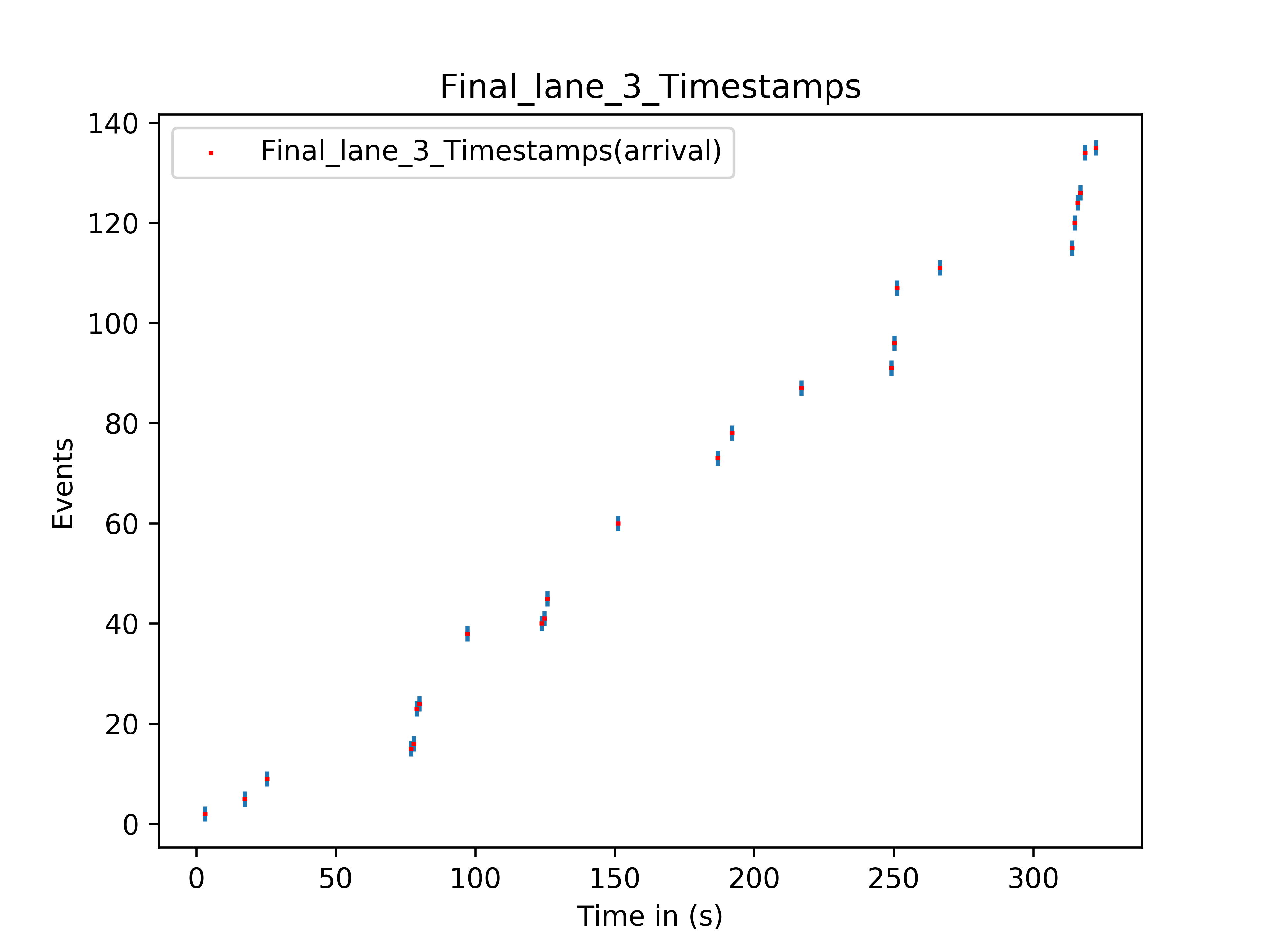
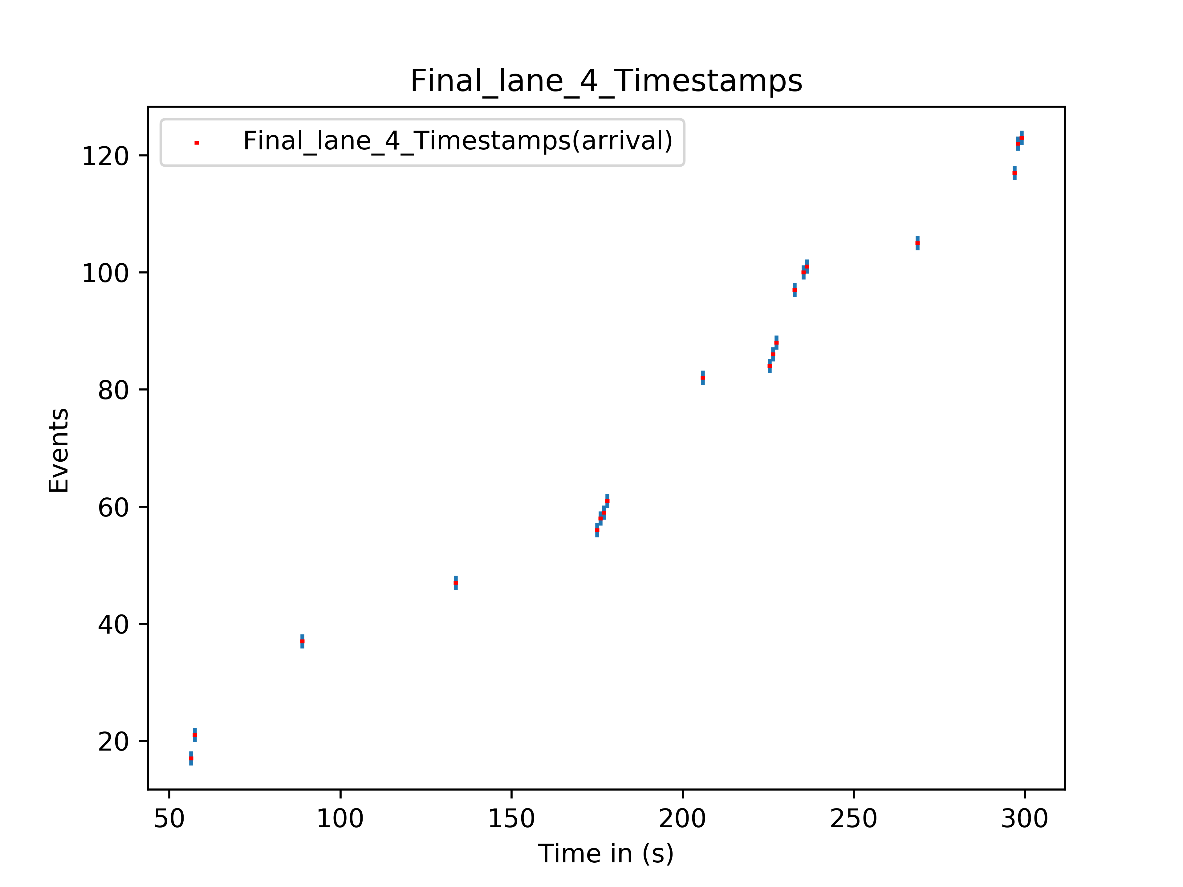
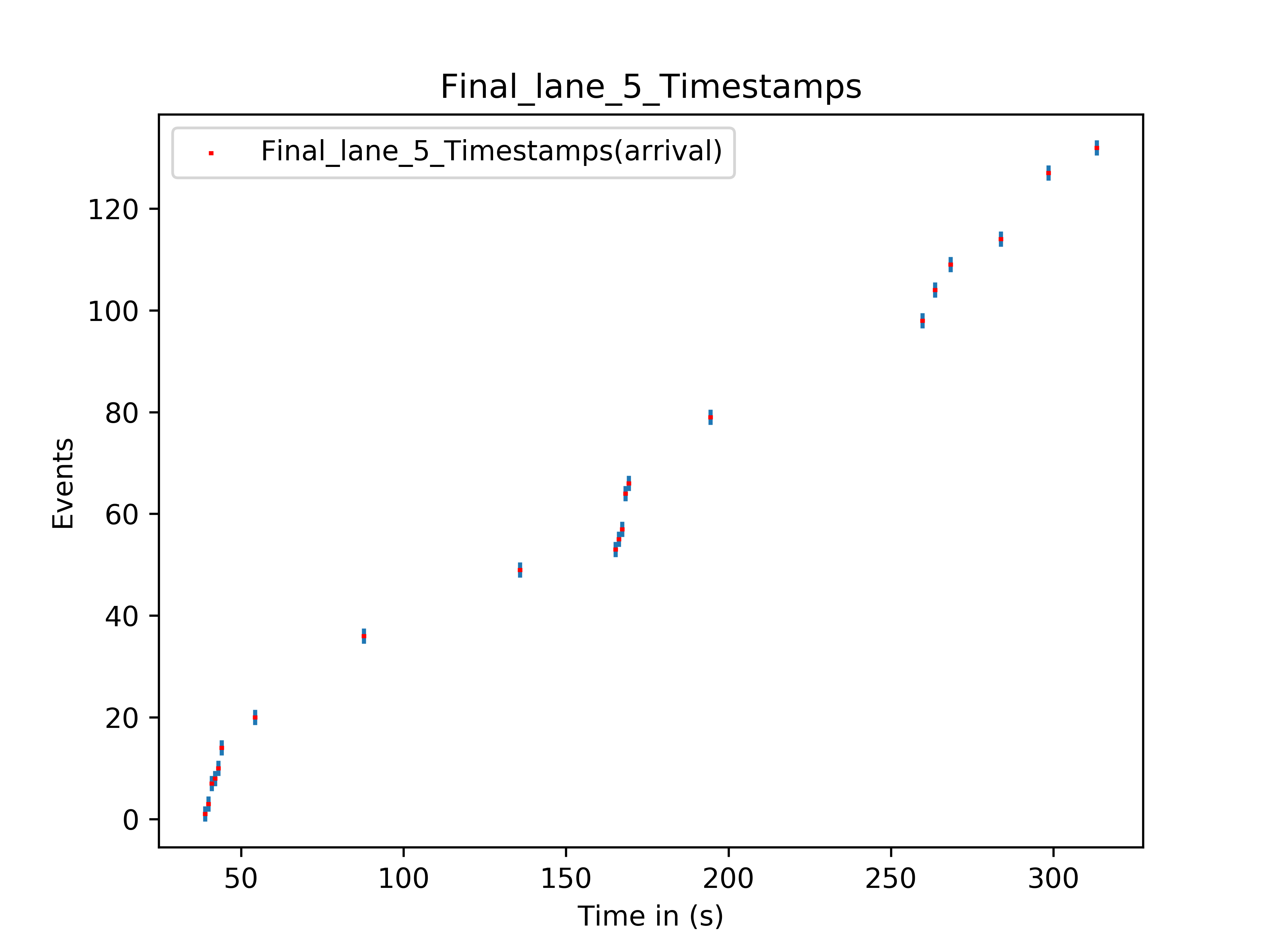
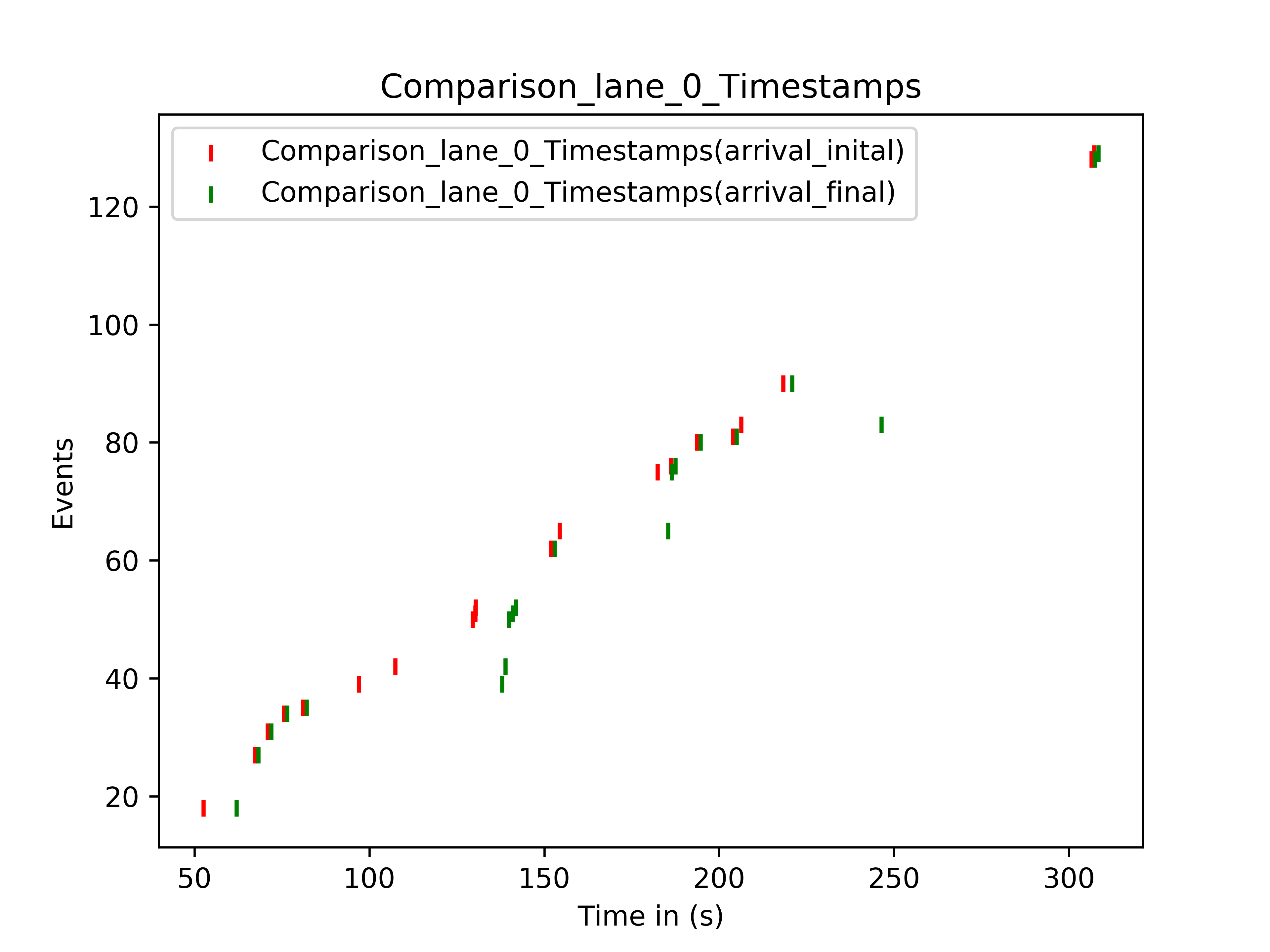
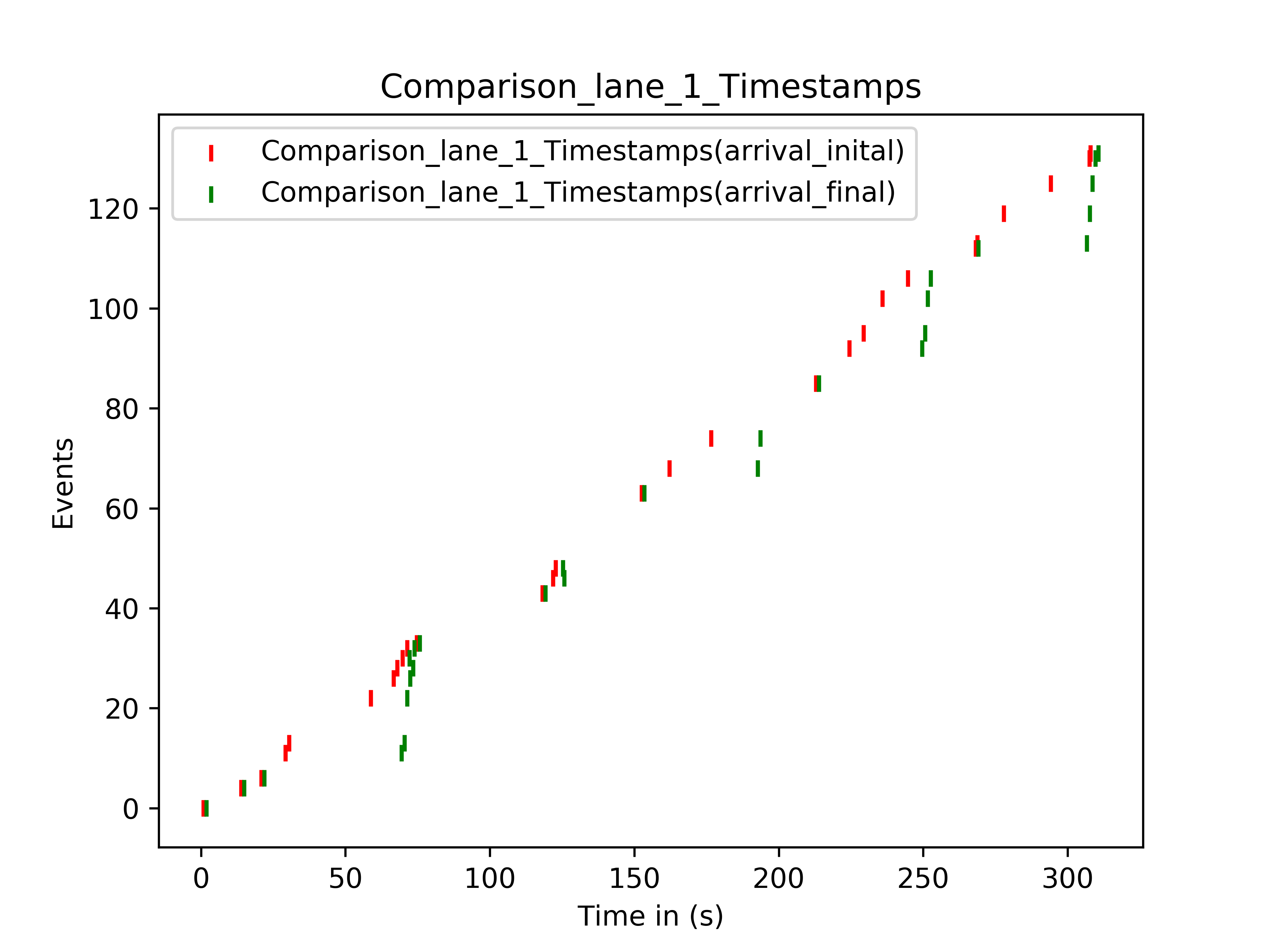
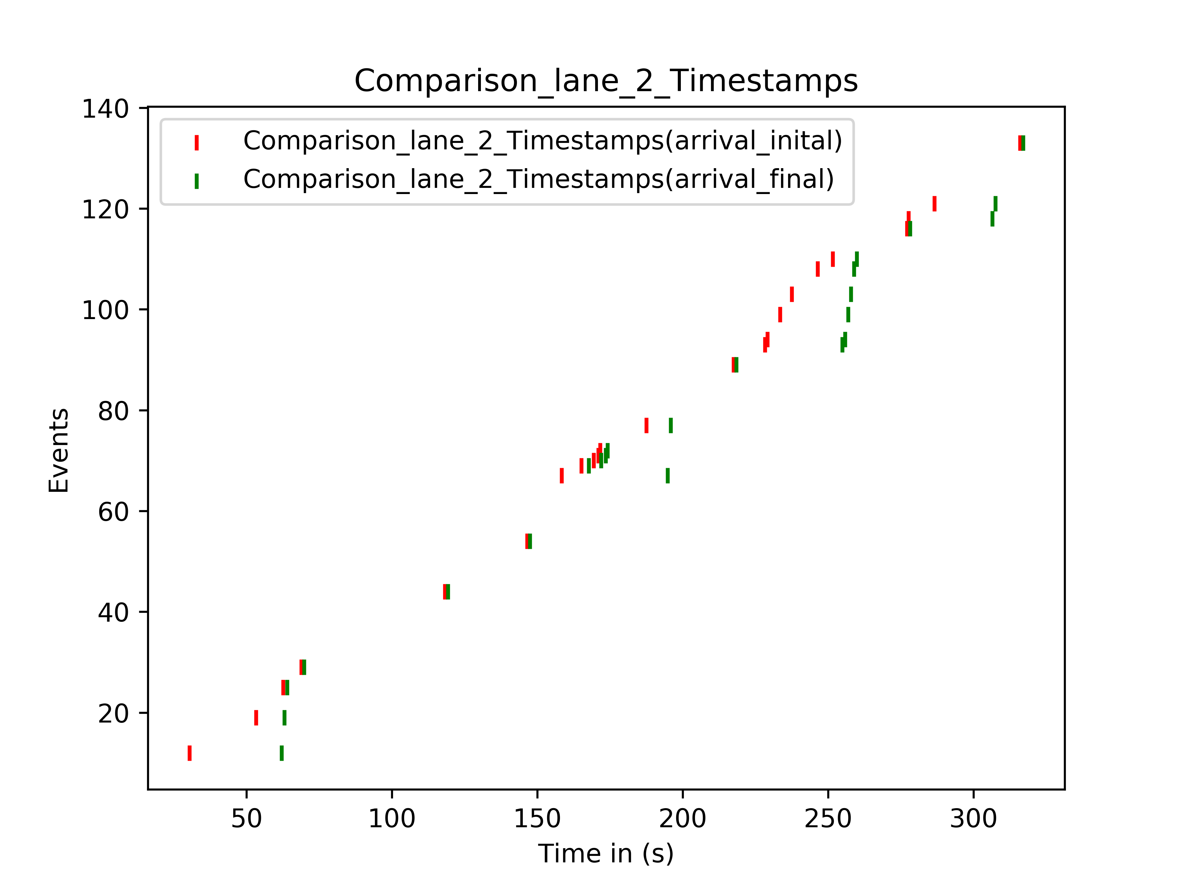
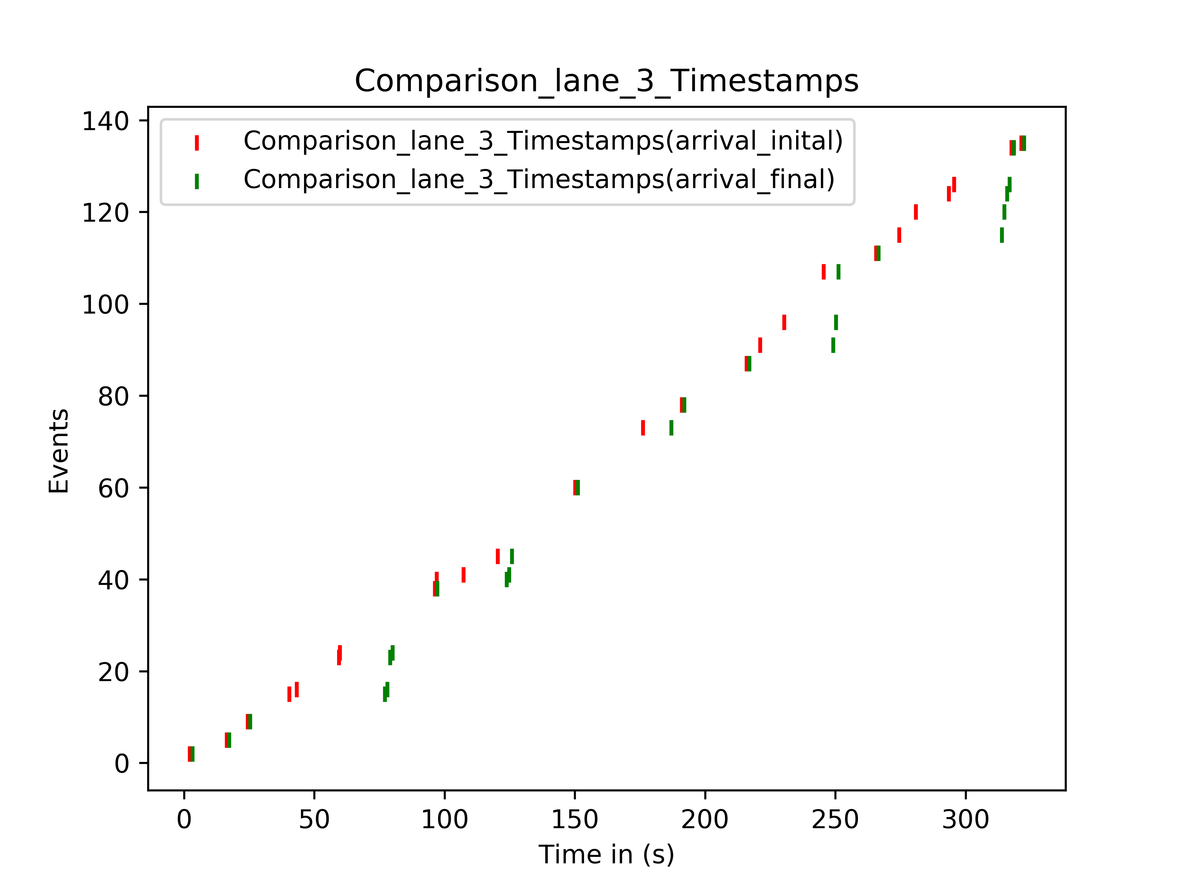
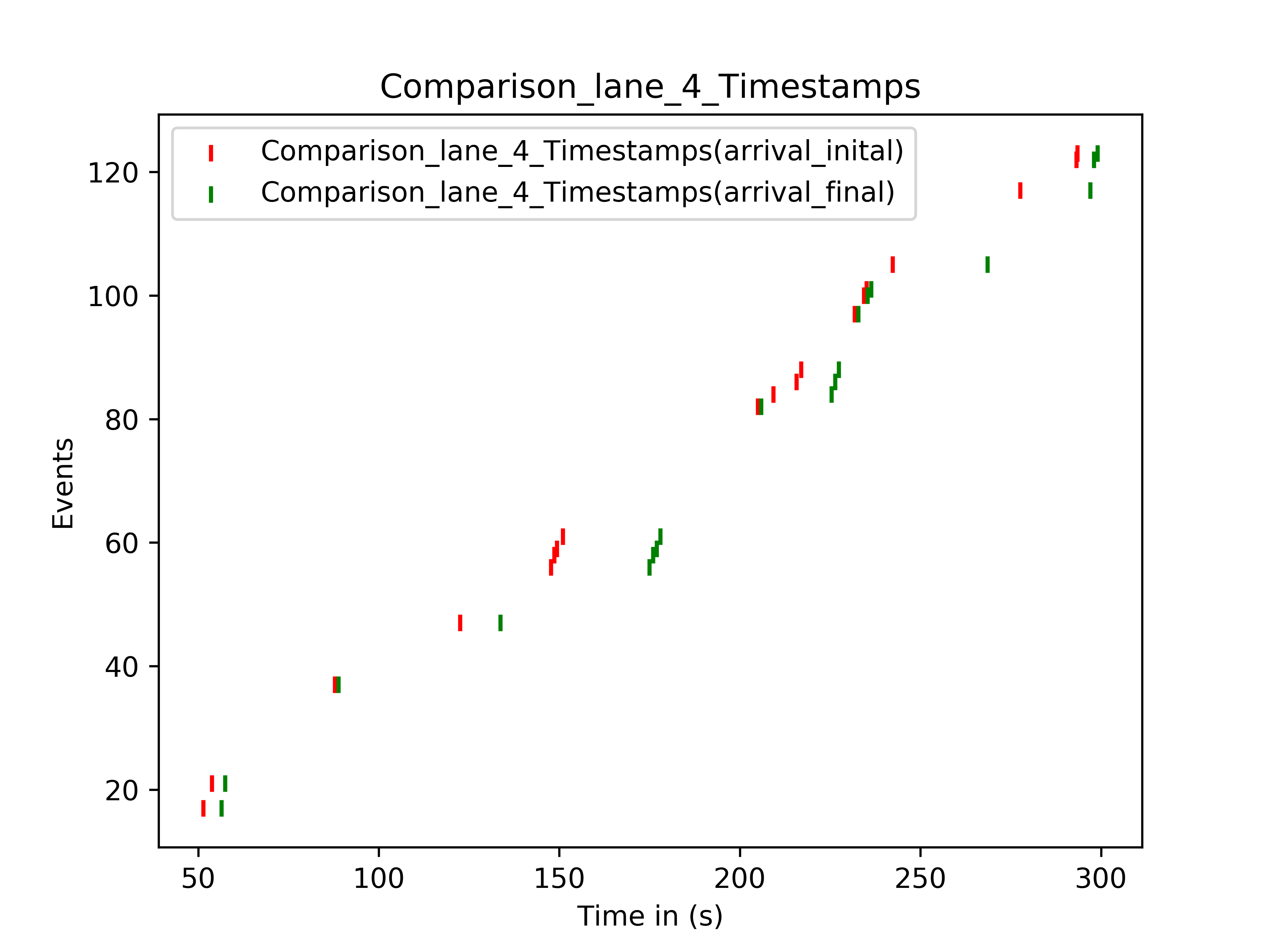
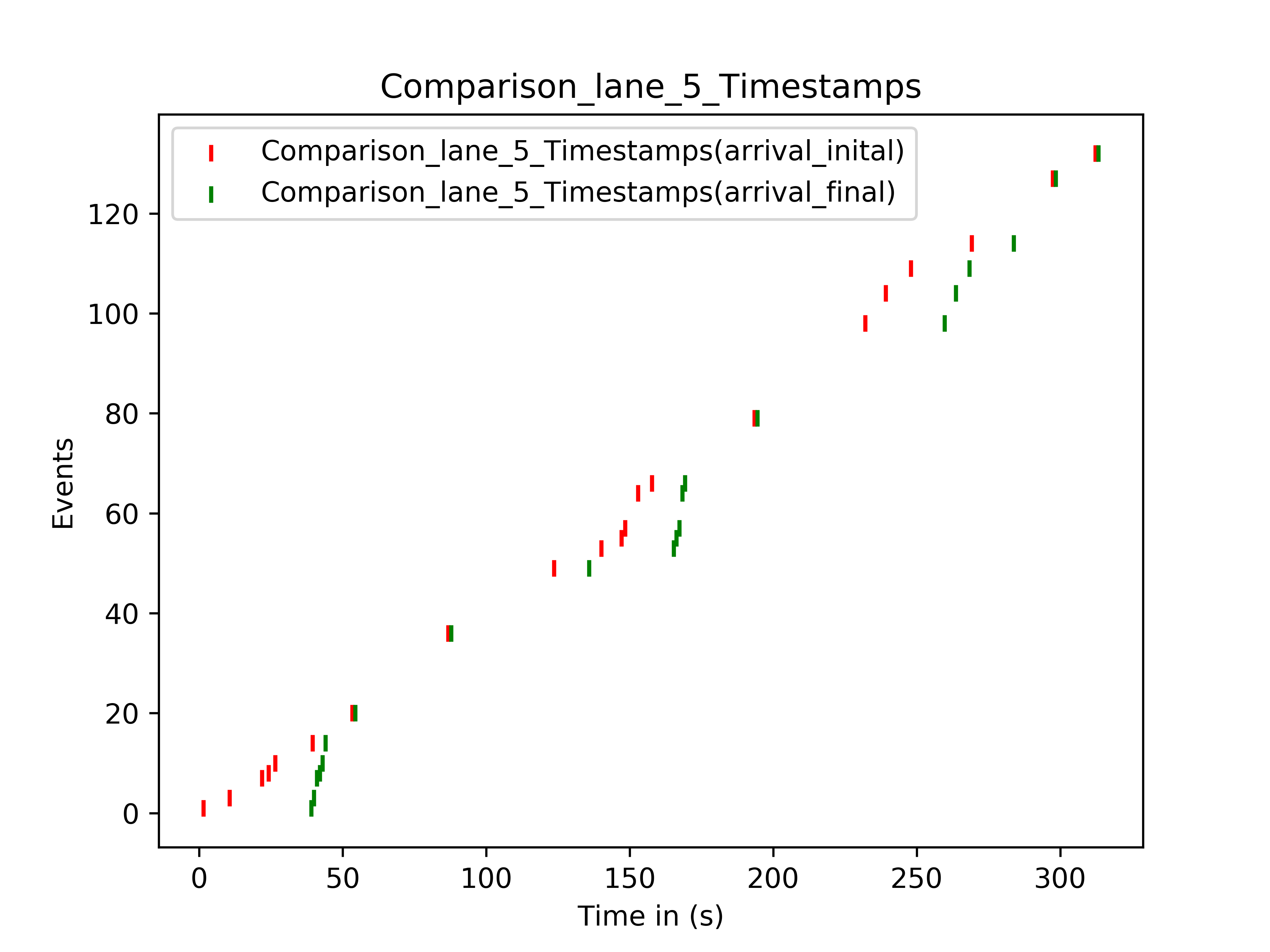
5. Comparision Each Lane Arrival Timestamps

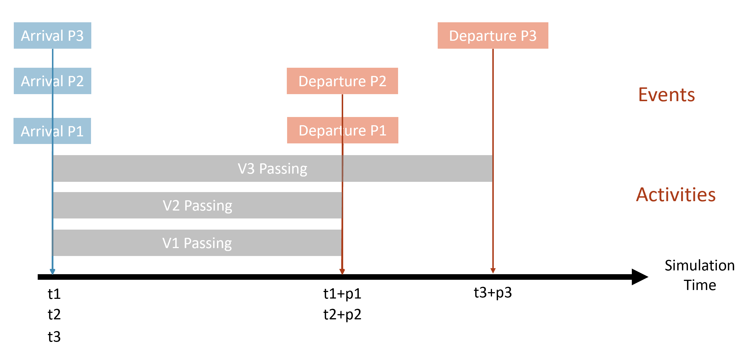
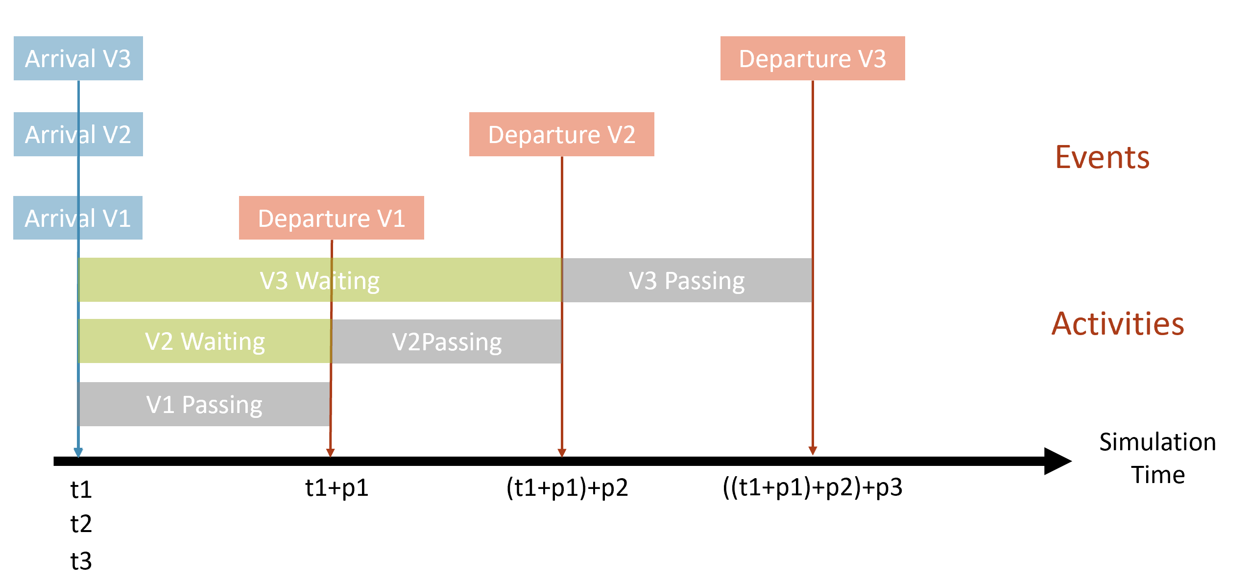
Discrete Event Flow Chart

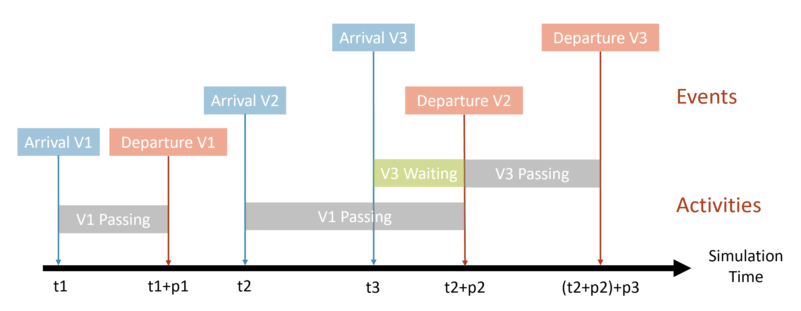
Visualization

Graphical playback of the simulation results can provide an intuitive and direct understanding of the discrete events happening. Although the events are discrete, we managed to visualize the simulation in continuous time span by placing the discrete time stamps into an unit time stepped visualization process. To achieve better playback visual effect, we chose to use javascript and react framework to render the events log in web browser. We chose to use deck.gl, a powerful open-sourced, web-GL based visualization platform to playback the logs.
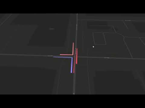
We added motion tracks to describe the car/pedestrain movements, mapped the event happening with real world longitude latitude coordinates in a zoomed interactive real map, by using mapbox’s service. Shown below is a screenshot of our visualization.

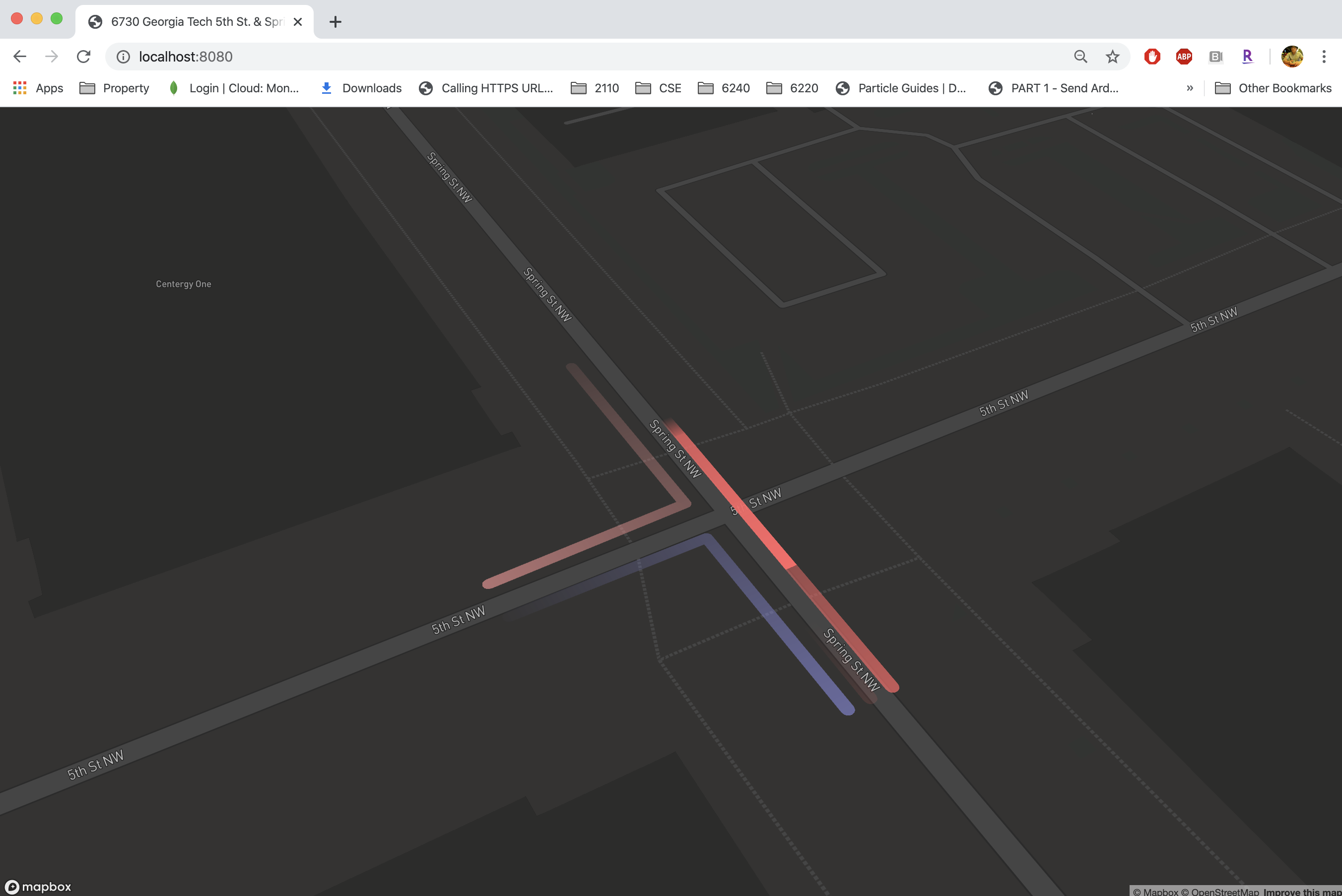
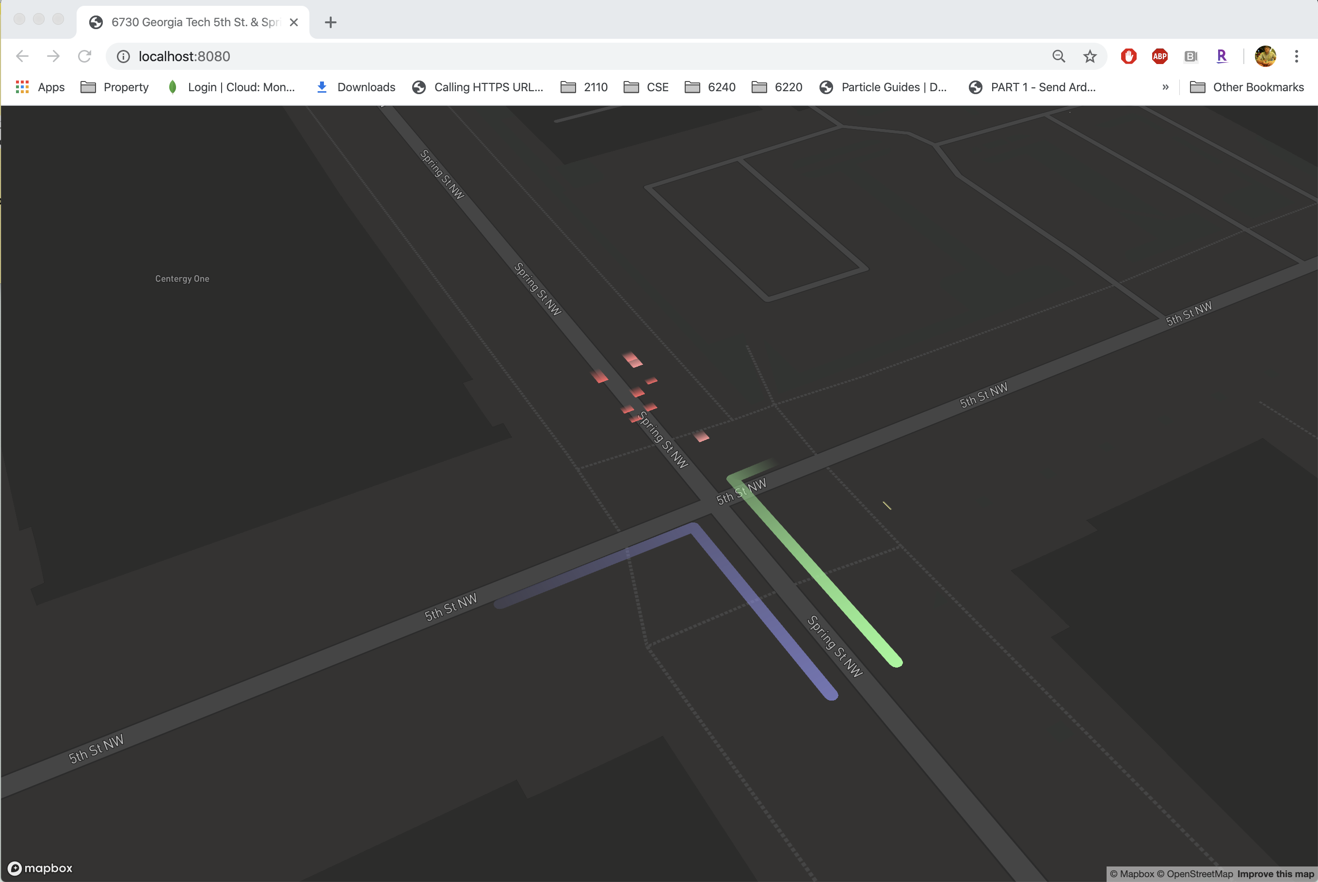
The web page is 3D and interactive, user can zoom, pan, rotate to view the playback from any angle. The camera auto focused to the tech square intersection location. We used different color scheme to differentiate the lanes, for example, North lane running towards are red, east lane is green, west lane is purple, pedestrian as yellow. We also use tail length of the car’s motion track to describe whether it is passing or waiting, waiting cars will have slow speed , short tails approaching to the intersection, while cars passing the intersection will have higher speed, longer tails motion track.

Video Demo

Result Table

Plese kindly visit out_sample.txt file to see the sample test results logs.

Analysis of Results

Please also see output figures section.

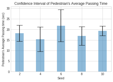
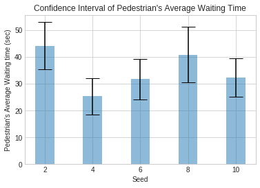
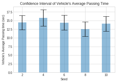
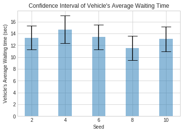
Besides, we performed a confidence level analysis by swapping different random generator seed numbers. The results shown below: